Simulated Annealing: Ising Model Project
— project, optimization, algorithms, physics — 14 min read
Note: The math behind the acceptance rule and cooling is in the companion post: Simulated Annealing: From Physics to Optimization.
Project Overview
I wanted something I could run and break: the Ising model is small enough to fit in a notebook, messy enough to feel real. Here is a brief summary of the project.
First we run Metropolis at a fixed temperature and see if the transition sits near the known $T_c$. If that fails, we have a problem.
Then we cool with simulated annealing on a 3D lattice and hunt for a low-energy state. In 2D we have Onsager’s number to compare against; in 3D we mostly have numerics: so we lean on the code and the plots.
Along the way: local $\Delta E$ updates, periodic boundaries, and the same acceptance rule as in the theory post.
1. The Ising Model: Quick Review
The Hamiltonian (Energy Function)
For a system of spins $\mathbf{s} = \{s_1, s_2, \ldots, s_N\}$ where each $s_i \in \{-1, +1\}$, the Ising Hamiltonian is:
E(\mathbf{s}) = -J \sum_{\langle i,j \rangle} s_i s_jKey components:
$J > 0$: Coupling constant (ferromagnetic: spins want to align)$\langle i,j \rangle$: Sum over nearest neighbors only- 2D: 4 neighbors per spin
- 3D: 6 neighbors per spin
$s_i s_j$: Interaction term- Aligned (
$s_i = s_j$): contributes$-J$(lower energy) - Anti-aligned (
$s_i \neq s_j$): contributes$+J$(higher energy)
- Aligned (
Ground State
The ground state (minimum energy) is when all spins are aligned:
- 2D:
$E_0 = -2JL^2$(per spin:$-2J$) - 3D:
$E_0 = -3JL^3$(per spin:$-3J$)
That gives us a simple scorecard when we run SA: how close did we get to all spins aligned?
Observables
- Energy:
$E = -J \sum_{\langle i,j \rangle} s_i s_j$ - Magnetization:
$M = \sum_i s_i$(sum of all spins) - Energy per spin:
$e = E / N$ - Magnetization per spin:
$m = M / N$
Phase Transitions
- Below
$T_c$: Ordered phase (high magnetization, low energy) - At
$T_c$: Critical point (phase transition) - Above
$T_c$: Disordered phase (low magnetization, higher energy)
Known critical temperatures:
- 2D: Exact solution by Onsager (1944)
$T_c / J = 2/\ln(1+\sqrt{2}) \approx 2.269$ - 3D: Well-characterized numerically
$T_c / J \approx 4.51$
Why the Ising Model Fits This Project
- We know the bottom in the ferromagnetic case (aligned spins), so we can tell if annealing helped or fooled us.
- The landscape is bumpy: domains and walls mean local minima show up without asking for them.
- Each move should stay cheap: updating one spin should not mean resumming the whole lattice (see §3).
2. The Critical Temperature (2D)
Onsager's Exact Solution
The 2D critical temperature is known in closed form (Onsager, 1944):
T_c = \frac{2J}{\ln(1 + \sqrt{2})} \approx 2.269 JThat value is the reference we use later when we check fixed-temperature Metropolis in 2D.
Deep Dive (Optional): Transfer Matrix and Where $T_c$ Comes From
Partition function
Computing $Z = \sum_{\{\mathbf{s}\}} e^{-E(\mathbf{s})/T}$ by brute force sums $2^{L^2}$ terms is not feasible for large $L$. The transfer-matrix approach builds $Z$ row by row instead of enumerating the full lattice at once.
Transfer matrix
For an $L \times L$ lattice, the transfer matrix $T$ is $2^L \times 2^L$: rows/columns index possible row configurations, and $T[i,j]$ stores the Boltzmann weight for transitioning from row $i$ to row $j$.
Trace formula
Z = \text{Tr}(T^N) = \sum_{i=1}^{2^L} \lambda_i^Nwhere $N$ is the number of rows and $\lambda_i$ are eigenvalues of $T$.
Complexity
- Direct sum:
$2^{L^2}$(exponential in area). - Transfer-matrix formulation: still exponential in the width
$L$, but structured enough to attack analytically.
Critical point
$T_c$ appears where the largest eigenvalue becomes degenerate (two eigenvalues equal). Carrying that out leads through the Onsager algebra: the non-commutative structure you get when the transfer matrix factors into pieces such as $T = V_1 V_2$ with $[V_1,V_2]\neq 0$. That is the algebraic backbone behind the closed form for $T_c$ in 2D.
3D: No Closed Form
There is no known closed-form thermodynamic solution for the standard 3D Ising model comparable to 2D. Practically:
- A transfer-matrix viewpoint blows up (exponential in cross-sectional area, not just width).
- Numerics give
$T_c / J \approx 4.51$for the cubic lattice (see references).
So for us, 3D is the part where we stop quoting closed forms and actually run the computational machinery.
3. Implementation Details
3.1 Fast Energy Calculation
The Problem: A full energy recomputation is $O(N)$ (each spin only talks to a few neighbors, but you still touch every spin). If you did that after every proposed flip in a sweep of $N$ proposals, a naive sweep would scale like $O(N^2)$.
The Solution: Track only the local energy change $\Delta E$ when flipping a single spin: $O(1)$ work per proposal if you sum neighbors only.
Derivation:
When we flip spin $s_i$:
- Before:
$E = -J \sum_{\langle i,j \rangle} s_i s_j + \text{(other terms)}$ - After:
$E' = -J \sum_{\langle i,j \rangle} (-s_i) s_j + \text{(other terms)}$
The change is:
\Delta E = E' - E = -J \sum_{j \in \text{nbrs}(i)} [(-s_i) s_j - s_i s_j] = -J \sum_{j \in \text{nbrs}(i)} [-2 s_i s_j] = 2J s_i \sum_{j \in \text{nbrs}(i)} s_jKey insight: Only the neighbors of the flipped spin contribute to the energy change!
Complexity: $O(1)$ per accepted/tested flip versus $O(N)$ for a full energy rebuild.
3.2 Periodic Boundary Conditions
Fixed boundaries give spins at the edge fewer neighbors than bulk spins. Periodic boundary conditions (PBC) remove that artifact by treating the lattice as a torus:
- Right edge connects to left edge
- Top edge connects to bottom edge
- In 3D: front connects to back
Topology: 2D torus; 3D hypertorus: every site sees the same neighborhood pattern.
Implementation (modulo indexing):
def get_neighbors(self, i, j, k): """PBC: (i+1) % L wraps around""" return [ self.spins[i, (j+1) % self.L, k], # Right neighbor self.spins[i, (j-1) % self.L, k], # Left neighbor self.spins[(i+1) % self.L, j, k], # Down neighbor self.spins[(i-1) % self.L, j, k], # Up neighbor self.spins[i, j, (k+1) % self.L], # Front neighbor self.spins[i, j, (k-1) % self.L] # Back neighbor ]Example: For $L=4$, spin at position $(3, 3)$:
- Right neighbor:
$(3, (3+1) \% 4) = (3, 0)$✔ (wraps to left) - Down neighbor:
$((3+1) \% 4, 3) = (0, 3)$✔ (wraps to top)
Result: Every spin has exactly the same number of neighbors, regardless of position!
3.3 From 2D to 3D: Code Portability
Key Insight: The code structure is nearly identical: only the neighbor count changes! This makes the code highly portable and easy to extend to higher dimensions.
Differences:
- Array dimensions:
$(L, L)$→$(L, L, L)$ - Neighbor count: 4 neighbors → 6 neighbors
- Energy per spin:
$-2J$→$-3J$(more neighbors = lower ground state energy) - Critical temperature:
$T_c \approx 2.27$→$T_c \approx 4.51$
What stays the same:
- Hamiltonian form:
$E = -J \sum_{\langle i,j \rangle} s_i s_j$ - Fast
$\Delta E$calculation: Same formula, just more neighbors - PBC implementation: Same modulo operator, just 3 dimensions
- Metropolis algorithm: Identical acceptance rule
4. Fixed-Temperature Metropolis Validation
Why Validate First?
Before cooling with SA, run Metropolis at fixed $T$ and check observables near $T_c$. If the phase transition lands in the wrong place, debugging SA first would waste time.
What "Fixed Temperature" Means Here
Hold $T$ constant for equilibration plus production sweeps so the chain samples roughly Boltzmann at that temperature; repeat across a temperature grid to cross the transition.
2D Validation
Runs at fixed $T$ near $T_c \approx 2.269$:
2D validation code — Ising2D, Metropolis sweep, fixed-T driver
class Ising2D: """2D Ising model with periodic boundary conditions.""" def __init__(self, L, J=1.0, random=True): self.L = L self.J = J self.N = L * L if random: self.spins = np.random.choice([-1, 1], size=(L, L)).astype(np.int8) else: self.spins = np.ones((L, L), dtype=np.int8) def get_neighbors(self, i, j): """Get 4 neighbors with PBC.""" return [ self.spins[i, (j+1) % self.L], # Right self.spins[i, (j-1) % self.L], # Left self.spins[(i+1) % self.L, j], # Down self.spins[(i-1) % self.L, j] # Up ] def delta_energy(self, i, j): """Fast energy change: O(1).""" neighbors = self.get_neighbors(i, j) sum_neighbors = sum(neighbors) return 2 * self.J * self.spins[i, j] * sum_neighbors def flip_spin(self, i, j): """Flip spin at (i, j).""" self.spins[i, j] *= -1 def get_energy(self): """Compute total energy.""" E = 0.0 for i in range(self.L): for j in range(self.L): neighbors = self.get_neighbors(i, j) E -= self.J * self.spins[i, j] * sum(neighbors) return E / 2 def get_energy_per_spin(self): return self.get_energy() / self.N def get_magnetization_per_spin(self): return abs(np.sum(self.spins)) / self.N
def metropolis_sweep_2d(ising, T, seed=None): """One Metropolis sweep (2D).""" if seed is not None: np.random.seed(seed) accepted = 0 for _ in range(ising.N): i = np.random.randint(0, ising.L) j = np.random.randint(0, ising.L) delta_E = ising.delta_energy(i, j) if delta_E < 0 or np.random.random() < np.exp(-delta_E / T): ising.flip_spin(i, j) accepted += 1 return accepted / ising.N
def run_fixed_T_2d(ising, T, n_sweeps, n_equil=100, seed=None): """Run Metropolis at fixed temperature T (2D).""" if seed is not None: np.random.seed(seed) # Equilibration for _ in range(n_equil): metropolis_sweep_2d(ising, T) # Production energies = [] magnetizations = [] for _ in range(n_sweeps): metropolis_sweep_2d(ising, T) energies.append(ising.get_energy_per_spin()) magnetizations.append(ising.get_magnetization_per_spin()) return { 'energies': np.array(energies), 'magnetizations': np.array(magnetizations) }Output:
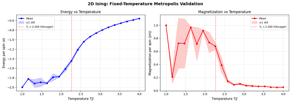
The curves line up with Onsager’s $T_c$: ordered side below $T_c$, disordered above, smooth energy crossing.
3D Validation
Same pipeline at $T_c \approx 4.51$. Code (full 3D lattice class):
3D validation code — Ising3D, Metropolis sweep, fixed-T driver
import numpy as npimport matplotlib.pyplot as pltfrom matplotlib.colors import ListedColormapfrom tqdm import tqdm
class Ising3D: """3D Ising model with periodic boundary conditions.""" def __init__(self, L, J=1.0, random=True): """Initialize 3D Ising lattice. Args: L: Linear size (L×L×L lattice) J: Coupling constant random: If True, random spins; if False, all +1 (ground state) """ self.L = L self.J = J self.N = L * L * L # Total number of spins # Initialize spins: 3D array of ±1 if random: self.spins = np.random.choice([-1, 1], size=(L, L, L)).astype(np.int8) else: self.spins = np.ones((L, L, L), dtype=np.int8) def get_neighbors(self, i, j, k): """Get 6 neighbors with periodic boundary conditions (PBC). Uses modulo operator: (i+1) % L automatically wraps around. """ neighbors = [] # 6 neighbors in 3D: ±x, ±y, ±z for di, dj, dk in [(-1,0,0), (1,0,0), (0,-1,0), (0,1,0), (0,0,-1), (0,0,1)]: ni = (i + di) % self.L # PBC: wraps around nj = (j + dj) % self.L nk = (k + dk) % self.L neighbors.append((ni, nj, nk)) return neighbors def delta_energy(self, i, j, k): """Fast energy change calculation: O(1) instead of O(N). Only neighbors contribute to energy change when flipping one spin. Formula: ΔE = 2J s_i Σ_j s_j (sum over neighbors) """ neighbors = self.get_neighbors(i, j, k) sum_neighbors = sum(self.spins[ni, nj, nk] for ni, nj, nk in neighbors) return 2 * self.J * self.spins[i, j, k] * sum_neighbors def flip_spin(self, i, j, k): """Flip spin at position (i, j, k).""" self.spins[i, j, k] *= -1 def get_energy(self): """Compute total energy (slow, for verification).""" E = 0.0 for i in range(self.L): for j in range(self.L): for k in range(self.L): neighbors = self.get_neighbors(i, j, k) for ni, nj, nk in neighbors: E -= self.J * self.spins[i, j, k] * self.spins[ni, nj, nk] return E / 2 # Divide by 2 to avoid double counting def get_energy_per_spin(self): """Get energy per spin.""" return self.get_energy() / self.N def get_magnetization_per_spin(self): """Get magnetization per spin.""" return np.sum(self.spins) / self.N def visualize_slice(self, axis=2, slice_idx=None, ax=None): """Visualize a 2D slice of the 3D configuration.""" if slice_idx is None: slice_idx = self.L // 2 if ax is None: fig, ax = plt.subplots(1, 1, figsize=(8, 8)) # Extract slice if axis == 0: slice_data = self.spins[slice_idx, :, :] elif axis == 1: slice_data = self.spins[:, slice_idx, :] else: slice_data = self.spins[:, :, slice_idx] cmap = ListedColormap(['blue', 'red']) im = ax.imshow(slice_data, cmap=cmap, vmin=-1, vmax=1) ax.set_title(f'3D Ising Slice (axis={axis}, slice={slice_idx})', fontsize=11) return ax
def metropolis_sweep_3d(ising, T, seed=None): """Perform one Metropolis sweep at temperature T (3D version). One sweep = N proposed spin flips (one per spin, in random order). """ if seed is not None: np.random.seed(seed) accepted = 0 # Propose N flips (one sweep) for _ in range(ising.N): # Random spin i = np.random.randint(0, ising.L) j = np.random.randint(0, ising.L) k = np.random.randint(0, ising.L) # Fast energy change calculation delta_E = ising.delta_energy(i, j, k) # Metropolis acceptance if delta_E < 0 or np.random.random() < np.exp(-delta_E / T): ising.flip_spin(i, j, k) accepted += 1 return accepted / ising.N
def run_fixed_T_3d(ising, T, n_sweeps, n_equil=100, seed=None): """Run Metropolis at fixed temperature T (3D).""" if seed is not None: np.random.seed(seed) # Equilibration for _ in range(n_equil): metropolis_sweep_3d(ising, T) # Production energies = [] magnetizations = [] for _ in range(n_sweeps): metropolis_sweep_3d(ising, T) energies.append(ising.get_energy_per_spin()) magnetizations.append(abs(ising.get_magnetization_per_spin())) return { 'energies': np.array(energies), 'magnetizations': np.array(magnetizations) }Output:
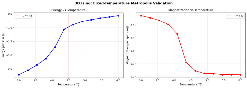
Qualitatively matches 2D; numerically pins $T_c$ where literature says it should be: excellent signal before SA.
5. Simulated Annealing for 3D Ising
Now we turn the dial: start hot so flips get accepted, then lower $T$ toward $T_{\min}$ and watch energy and acceptance along the way. The goal is a cheap path to a very low energy: not a proof, just a good final lattice.
SA Implementation
We'll use a geometric cooling schedule: $T_{k+1} = \alpha T_k$ where $\alpha = 0.98$ (slow cooling).
Simulated annealing code — geometric schedule + simulated_annealing_3d
class GeometricSchedule: """Geometric cooling schedule: T_{k+1} = alpha * T_k""" def __init__(self, T0, T_min, alpha=0.95): self.T0 = T0 self.T_min = T_min self.alpha = alpha self.T = T0 self.k = 0 def get_temperature(self): return self.T def cool(self): self.T = max(self.T * self.alpha, self.T_min) self.k += 1 def is_done(self): return self.T <= self.T_min
def simulated_annealing_3d(ising, schedule, sweeps_per_T=10, seed=None): """Run Simulated Annealing on 3D Ising model. Args: ising: Ising3D instance schedule: Cooling schedule (GeometricSchedule) sweeps_per_T: Number of sweeps at each temperature seed: Random seed Returns: Dictionary with history (energies, temperatures, acceptance_rates) """ if seed is not None: np.random.seed(seed) energies = [] temperatures = [] acceptance_rates = [] while not schedule.is_done(): T = schedule.get_temperature() # Run sweeps at this temperature for _ in range(sweeps_per_T): acc_rate = metropolis_sweep_3d(ising, T) energies.append(ising.get_energy_per_spin()) temperatures.append(T) acceptance_rates.append(acc_rate) schedule.cool() return { 'energies': np.array(energies), 'temperatures': np.array(temperatures), 'acceptance_rates': np.array(acceptance_rates) }Running SA
L = 12 # System sizeJ = 1.0T0 = 6.0 # High starting temperatureT_min = 0.2alpha = 0.98 # Slow coolingsweeps_per_T = 10
# Ground state energy per spinE_ground = -3 * J # All spins aligned in 3D
# Create systemising = Ising3D(L, J=J, random=True)E_init = ising.get_energy_per_spin()
# Run SAschedule = GeometricSchedule(T0, T_min, alpha=alpha)results = simulated_annealing_3d(ising, schedule, sweeps_per_T=sweeps_per_T, seed=42)
E_final = ising.get_energy_per_spin()Output:
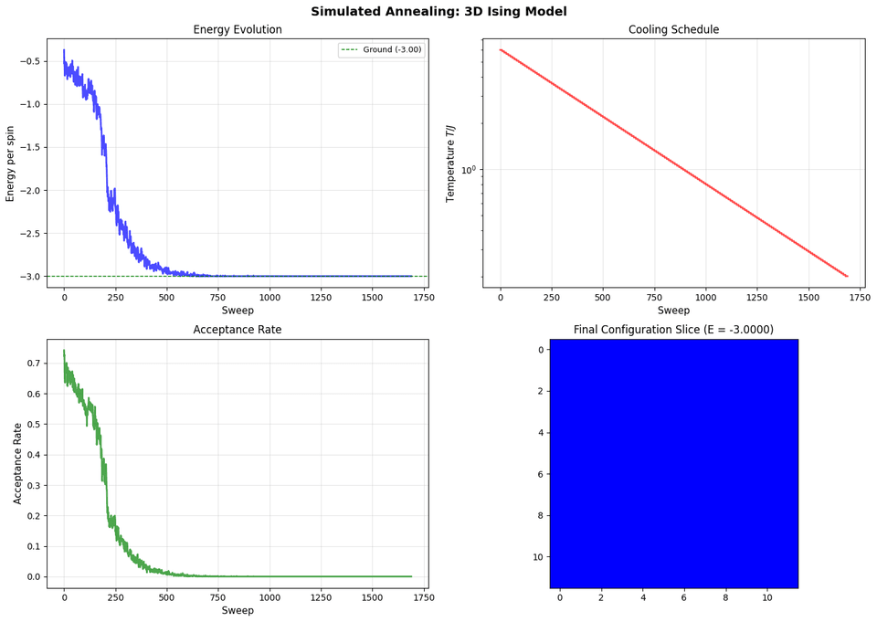
Reading the Run
Energy tends to drift down as $T$ drops. Early on the acceptance rate stays high: the lattice still explores. Later it gets picky, as it should. If you watch slices of the lattice, you can see little islands at hot $T$ turn into big patches as $T$ falls: same picture as in the theory post, but this time is real data.
6. Closing
Simulated annealing is still only Metropolis with a temperature that drops. The difference is we give the system room to walk around while $T$ is high, then let it settle when $T$ is low.
I did not tune this run to death: other $L$, $\alpha$, seeds, and schedules will behave differently. That is fine.
What matters to me is that we used a simulation to check the physics first: does the transition land near $T_c$ where it should? Once that looked right, we could trust the same machinery in a harder setting (3D), where there is no tidy closed form to lean on, and still run simulated annealing as an optimizer rather than a guess.
That finishes the loop for me: theory in the companion post, plots that behave like the textbooks, then practice in code.
References
-
Onsager, L. (1944). Crystal statistics. I. A two-dimensional model with an order-disorder transition. Physical Review, 65(3-4), 117-149. — Exact solution for 2D Ising model
-
Binder, K., & Heermann, D. W. (2010). Monte Carlo Simulation in Statistical Physics: An Introduction. Springer. — 3D Ising critical temperature
$T_c / J \approx 4.51$ -
Kirkpatrick, S., Gelatt, C. D., & Vecchi, M. P. (1983). Optimization by simulated annealing. Science, 220(4598), 671-680. — Original Simulated Annealing paper
-
Metropolis, N., et al. (1953). Equation of state calculations by fast computing machines. The Journal of Chemical Physics, 21(6), 1087-1092. — Original Metropolis algorithm