Simulated Annealing: Ising Model Project

05.01.2026 — project, optimization, algorithms, physics — 15 min read

Note: For the theoretical foundations of Simulated Annealing, see the companion blog post: Simulated Annealing: From Physics to Optimization

Project Overview

This project demonstrates Simulated Annealing applied to the Ising Model: a classic problem in statistical physics that is an ideal testbed for Simulated Annealing

What You'll Learn:

Why the Ising model is perfect for demonstrating SA
Onsager's exact solution for 2D Ising (one of the most beautiful results in physics)
Implementation techniques: fast energy calculation, periodic boundary conditions
How SA successfully optimizes the 3D Ising model

1. The Ising Model: Quick Review

The Hamiltonian (Energy Function)

For a system of spins $\mathbf{s} = \{s_1, s_2, \ldots, s_N\}$ where each $s_i \in \{-1, +1\}$ , the Ising Hamiltonian is:

E(\mathbf{s}) = -J \sum_{\langle i,j \rangle} s_i s_j

Key components:

$J > 0$ : Coupling constant (ferromagnetic: spins want to align)
$\langle i,j \rangle$ : Sum over nearest neighbors only
- 2D: 4 neighbors per spin
- 3D: 6 neighbors per spin
$s_i s_j$ : Interaction term
- Aligned ( $s_i = s_j$ ): contributes $-J$ (lower energy)
- Anti-aligned ( $s_i \neq s_j$ ): contributes $+J$ (higher energy)

Ground State

The ground state (minimum energy) is when all spins are aligned:

2D: $E_0 = -2JL^2$ (per spin: $-2J$ )
3D: $E_0 = -3JL^3$ (per spin: $-3J$ )

This well-defined ground state makes it easy to evaluate how well SA performs.

Observables

Energy: $E = -J \sum_{\langle i,j \rangle} s_i s_j$
Magnetization: $M = \sum_i s_i$ (sum of all spins)
Energy per spin: $e = E / N$
Magnetization per spin: $m = M / N$

Phase Transitions

Below $T_c$ : Ordered phase (high magnetization, low energy)
At $T_c$ : Critical point (phase transition)
Above $T_c$ : Disordered phase (low magnetization, higher energy)

Known critical temperatures:

2D: Exact solution by Onsager (1944) — $T_c / J = 2/\ln(1+\sqrt{2}) \approx 2.269$
3D: Well-characterized numerically — $T_c / J \approx 4.51$

Why Ising Model is Perfect for SA

The Ising model serves as an excellent benchmark for Simulated Annealing because:

Clear optimization goal: The ground state (all spins aligned) is known, making it easy to evaluate SA's performance
Many local minima: Different spin configurations with varying energies create a challenging optimization landscape
Energy barriers: The system needs thermal fluctuations to escape local minima, which is exactly what SA provides
Visualizable: In 2D and 3D, we can visualize spin configurations, see domains form and grow, and observe how SA explores the energy landscape
Scalable: We can study systems from small ( $L=8$ ) for debugging to large ( $L=32+$ ) for realistic physics
Well-characterized: Extensive literature and known results (especially Onsager's exact 2D solution) provide validation benchmarks

2. The Critical Temperature (2D)

Onsager's Exact Solution

The critical temperature for the 2D Ising model is a remarkable exact result derived by Lars Onsager in 1944:

T_c = \frac{2J}{\ln(1 + \sqrt{2})} \approx 2.269 J

Most models require numerical methods or approximations, but Onsager's exact analytical solution reveals deep mathematical structure (the Onsager algebra) and provides a crucial benchmark for validating numerical methods.

This is a good example of how hidden symmetries can make exact solutions possible.

Sketch of Onsager's Solution

Onsager's solution uses the transfer matrix method, which reduces the 2D problem to a 1D eigenvalue problem. Here's the key idea:

The Challenge: Computing the partition function $Z = \sum_{\{\mathbf{s}\}} e^{-E(\mathbf{s})/T}$ requires summing over $2^{L^2}$ configurations—impossible for large $L$ !

The Breakthrough: Instead of summing over all configurations at once, build the partition function row by row using a transfer matrix.

The Transfer Matrix:

For an $L \times L$ lattice, the transfer matrix $T$ is $2^L \times 2^L$
Each row/column corresponds to one of the $2^L$ possible row configurations
Matrix element $T[i,j]$ encodes the Boltzmann weight for transitioning from row configuration $i$ to row configuration $j$

The Magic: The partition function becomes:

Z = \text{Tr}(T^N) = \sum_{i=1}^{2^L} \lambda_i^N

where $N$ is the number of rows and $\lambda_i$ are eigenvalues of $T$ .

Complexity Reduction:

Direct sum: $2^{L^2}$ terms (exponential in area)
Transfer matrix: $2^L \times 2^L$ matrix (exponential in width, not area!)

Finding $T_c$ : The critical temperature occurs when the largest eigenvalue becomes degenerate (two eigenvalues become equal). This requires solving the Onsager algebra—a non-commutative Lie algebra that describes the symmetries of the 2D Ising model.

Why Onsager Algebra? The transfer matrix can be written as $T = V_1 V_2$ where $V_1$ and $V_2$ don't commute. The Onsager algebra provides the mathematical structure needed to diagonalize this and find the eigenvalues exactly.

The Result: After solving the Onsager algebra, the critical temperature emerges as:

T_c = \frac{2J}{\ln(1 + \sqrt{2})}

This is why physicists learn group theory and Lie algebras—they reveal hidden symmetries that make exact solutions possible!

3D Case: No Exact Solution

For the 3D Ising model, there is no known exact solution. This is one of the most famous open problems in statistical physics!

Why is 3D harder?

Transfer matrix would be $2^{L^2} \times 2^{L^2}$ (exponential in area, not just width)
The Onsager algebra structure doesn't generalize to 3D
No exact solution has been found despite decades of effort

What we know:

Critical temperature: $T_c / J \approx 4.51$ (from numerical methods)
Phase transition exists and is well-characterized
But no closed-form formula like the 2D case

This makes the 3D Ising model a perfect test case for numerical methods like Simulated Annealing!

3. Implementation Details

3.1 Fast Energy Calculation

The Problem: Recomputing the total energy after each spin flip would be $O(N^2)$ . This is too slow for large systems!

The Solution: Compute only the local energy change $\Delta E$ when flipping a single spin.

Derivation:

When we flip spin $s_i$ :

Before: $E = -J \sum_{\langle i,j \rangle} s_i s_j + \text{(other terms)}$
After: $E' = -J \sum_{\langle i,j \rangle} (-s_i) s_j + \text{(other terms)}$

The change is:

\Delta E = E' - E = -J \sum_{j \in \text{nbrs}(i)} [(-s_i) s_j - s_i s_j] = -J \sum_{j \in \text{nbrs}(i)} [-2 s_i s_j] = 2J s_i \sum_{j \in \text{nbrs}(i)} s_j

Key insight: Only the neighbors of the flipped spin contribute to the energy change!

Complexity: $O(1)$ per flip (only need to sum over neighbors) vs $O(N)$ for full recomputation.

3.2 Periodic Boundary Conditions

Why Needed: Fixed boundaries create edge effects. Spins at edges have fewer neighbors, which doesn't reflect the thermodynamic limit.

The Solution: Periodic boundary conditions (PBC) treat the lattice as a torus:

Right edge connects to left edge
Top edge connects to bottom edge
In 3D: front connects to back

Topology:

2D: Torus (donut shape)
3D: Hypertorus

Why Torus? Topologically, a torus has no boundaries: every point is equivalent. This eliminates edge effects and provides translation invariance.

Implementation: Use the modulo operator:

def get_neighbors(self, i, j, k):
    """PBC: (i+1) % L wraps around"""
    return [
        self.spins[i, (j+1) % self.L, k],      # Right neighbor
        self.spins[i, (j-1) % self.L, k],      # Left neighbor
        self.spins[(i+1) % self.L, j, k],      # Down neighbor
        self.spins[(i-1) % self.L, j, k],      # Up neighbor
        self.spins[i, j, (k+1) % self.L],      # Front neighbor
        self.spins[i, j, (k-1) % self.L]       # Back neighbor
    ]

Example: For $L=4$ , spin at position $(3, 3)$ :

Right neighbor: $(3, (3+1) \% 4) = (3, 0)$ ✔ (wraps to left)
Down neighbor: $((3+1) \% 4, 3) = (0, 3)$ ✔ (wraps to top)

Result: Every spin has exactly the same number of neighbors, regardless of position!

3.3 From 2D to 3D: Code Portability

Key Insight: The code structure is nearly identical: only the neighbor count changes! This makes the code highly portable and easy to extend to higher dimensions.

Differences:

Array dimensions: $(L, L)$ → $(L, L, L)$
Neighbor count: 4 neighbors → 6 neighbors
Energy per spin: $-2J$ → $-3J$ (more neighbors = lower ground state energy)
Critical temperature: $T_c \approx 2.27$ → $T_c \approx 4.51$

What stays the same:

Hamiltonian form: $E = -J \sum_{\langle i,j \rangle} s_i s_j$
Fast $\Delta E$ calculation: Same formula, just more neighbors
PBC implementation: Same modulo operator, just 3 dimensions
Metropolis algorithm: Identical acceptance rule

4. Fixed-Temperature Metropolis Validation

Why Validate First?

Before using SA for optimization, we need to validate that our implementation produces correct physics. This ensures:

Our code is correct
The phase transition occurs at the expected $T_c$
We can trust our SA results

What is "Fixed Temperature"?

Fixed temperature means we run the Metropolis algorithm at a constant temperature $T$ for many sweeps. The system reaches thermal equilibrium at that temperature, sampling from the Boltzmann distribution.

We test at multiple different temperatures (low, medium, high) to see how the system behaves across the phase transition.

2D Validation

Let's validate our 2D implementation by checking the phase transition near $T_c \approx 2.269$ :

class Ising2D:
    """2D Ising model with periodic boundary conditions."""
    
    def __init__(self, L, J=1.0, random=True):
        self.L = L
        self.J = J
        self.N = L * L
        
        if random:
            self.spins = np.random.choice([-1, 1], size=(L, L)).astype(np.int8)
        else:
            self.spins = np.ones((L, L), dtype=np.int8)
    
    def get_neighbors(self, i, j):
        """Get 4 neighbors with PBC."""
        return [
            self.spins[i, (j+1) % self.L],  # Right
            self.spins[i, (j-1) % self.L],  # Left
            self.spins[(i+1) % self.L, j],  # Down
            self.spins[(i-1) % self.L, j]   # Up
        ]
    
    def delta_energy(self, i, j):
        """Fast energy change: O(1)."""
        neighbors = self.get_neighbors(i, j)
        sum_neighbors = sum(neighbors)
        return 2 * self.J * self.spins[i, j] * sum_neighbors
    
    def flip_spin(self, i, j):
        """Flip spin at (i, j)."""
        self.spins[i, j] *= -1
    
    def get_energy(self):
        """Compute total energy."""
        E = 0.0
        for i in range(self.L):
            for j in range(self.L):
                neighbors = self.get_neighbors(i, j)
                E -= self.J * self.spins[i, j] * sum(neighbors)
        return E / 2
    
    def get_energy_per_spin(self):
        return self.get_energy() / self.N
    
    def get_magnetization_per_spin(self):
        return abs(np.sum(self.spins)) / self.N


def metropolis_sweep_2d(ising, T, seed=None):
    """One Metropolis sweep (2D)."""
    if seed is not None:
        np.random.seed(seed)
    
    accepted = 0
    for _ in range(ising.N):
        i = np.random.randint(0, ising.L)
        j = np.random.randint(0, ising.L)
        delta_E = ising.delta_energy(i, j)
        if delta_E < 0 or np.random.random() < np.exp(-delta_E / T):
            ising.flip_spin(i, j)
            accepted += 1
    return accepted / ising.N


def run_fixed_T_2d(ising, T, n_sweeps, n_equil=100, seed=None):
    """Run Metropolis at fixed temperature T (2D)."""
    if seed is not None:
        np.random.seed(seed)
    
    # Equilibration
    for _ in range(n_equil):
        metropolis_sweep_2d(ising, T)
    
    # Production
    energies = []
    magnetizations = []
    for _ in range(n_sweeps):
        metropolis_sweep_2d(ising, T)
        energies.append(ising.get_energy_per_spin())
        magnetizations.append(ising.get_magnetization_per_spin())
    
    return {
        'energies': np.array(energies),
        'magnetizations': np.array(magnetizations)
    }

Output:

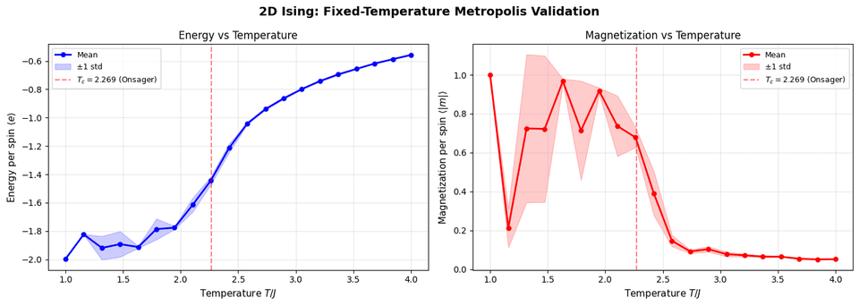
Running this validation shows that:

Phase transition occurs near $T_c \approx 2.269$ (Onsager's exact result)
Low T: High magnetization (ordered phase)
High T: Low magnetization (disordered phase)
Energy increases smoothly with T

3D Validation

The same validation procedure works for 3D, just with a different critical temperature ( $T_c \approx 4.51$ ). The physics is the same: we're just checking that our 3D implementation produces the correct phase transition.

Here's the complete 3D Ising model implementation:

import numpy as np
import matplotlib.pyplot as plt
from matplotlib.colors import ListedColormap
from tqdm import tqdm

class Ising3D:
    """3D Ising model with periodic boundary conditions."""
    
    def __init__(self, L, J=1.0, random=True):
        """Initialize 3D Ising lattice.
        
        Args:
            L: Linear size (L×L×L lattice)
            J: Coupling constant
            random: If True, random spins; if False, all +1 (ground state)
        """
        self.L = L
        self.J = J
        self.N = L * L * L  # Total number of spins
        
        # Initialize spins: 3D array of ±1
        if random:
            self.spins = np.random.choice([-1, 1], size=(L, L, L)).astype(np.int8)
        else:
            self.spins = np.ones((L, L, L), dtype=np.int8)
    
    def get_neighbors(self, i, j, k):
        """Get 6 neighbors with periodic boundary conditions (PBC).
        
        Uses modulo operator: (i+1) % L automatically wraps around.
        """
        neighbors = []
        # 6 neighbors in 3D: ±x, ±y, ±z
        for di, dj, dk in [(-1,0,0), (1,0,0), (0,-1,0), (0,1,0), (0,0,-1), (0,0,1)]:
            ni = (i + di) % self.L  # PBC: wraps around
            nj = (j + dj) % self.L
            nk = (k + dk) % self.L
            neighbors.append((ni, nj, nk))
        return neighbors
    
    def delta_energy(self, i, j, k):
        """Fast energy change calculation: O(1) instead of O(N).
        
        Only neighbors contribute to energy change when flipping one spin.
        Formula: ΔE = 2J s_i Σ_j s_j (sum over neighbors)
        """
        neighbors = self.get_neighbors(i, j, k)
        sum_neighbors = sum(self.spins[ni, nj, nk] for ni, nj, nk in neighbors)
        return 2 * self.J * self.spins[i, j, k] * sum_neighbors
    
    def flip_spin(self, i, j, k):
        """Flip spin at position (i, j, k)."""
        self.spins[i, j, k] *= -1
    
    def get_energy(self):
        """Compute total energy (slow, for verification)."""
        E = 0.0
        for i in range(self.L):
            for j in range(self.L):
                for k in range(self.L):
                    neighbors = self.get_neighbors(i, j, k)
                    for ni, nj, nk in neighbors:
                        E -= self.J * self.spins[i, j, k] * self.spins[ni, nj, nk]
        return E / 2  # Divide by 2 to avoid double counting
    
    def get_energy_per_spin(self):
        """Get energy per spin."""
        return self.get_energy() / self.N
    
    def get_magnetization_per_spin(self):
        """Get magnetization per spin."""
        return np.sum(self.spins) / self.N
    
    def visualize_slice(self, axis=2, slice_idx=None, ax=None):
        """Visualize a 2D slice of the 3D configuration."""
        if slice_idx is None:
            slice_idx = self.L // 2
        
        if ax is None:
            fig, ax = plt.subplots(1, 1, figsize=(8, 8))
        
        # Extract slice
        if axis == 0:
            slice_data = self.spins[slice_idx, :, :]
        elif axis == 1:
            slice_data = self.spins[:, slice_idx, :]
        else:
            slice_data = self.spins[:, :, slice_idx]
        
        cmap = ListedColormap(['blue', 'red'])
        im = ax.imshow(slice_data, cmap=cmap, vmin=-1, vmax=1)
        ax.set_title(f'3D Ising Slice (axis={axis}, slice={slice_idx})', fontsize=11)
        return ax


def metropolis_sweep_3d(ising, T, seed=None):
    """Perform one Metropolis sweep at temperature T (3D version).
    
    One sweep = N proposed spin flips (one per spin, in random order).
    """
    if seed is not None:
        np.random.seed(seed)
    
    accepted = 0
    
    # Propose N flips (one sweep)
    for _ in range(ising.N):
        # Random spin
        i = np.random.randint(0, ising.L)
        j = np.random.randint(0, ising.L)
        k = np.random.randint(0, ising.L)
        
        # Fast energy change calculation
        delta_E = ising.delta_energy(i, j, k)
        
        # Metropolis acceptance
        if delta_E < 0 or np.random.random() < np.exp(-delta_E / T):
            ising.flip_spin(i, j, k)
            accepted += 1
    
    return accepted / ising.N

def run_fixed_T_3d(ising, T, n_sweeps, n_equil=100, seed=None):
    """Run Metropolis at fixed temperature T (3D)."""
    if seed is not None:
        np.random.seed(seed)
    
    # Equilibration
    for _ in range(n_equil):
        metropolis_sweep_3d(ising, T)
    
    # Production
    energies = []
    magnetizations = []
    for _ in range(n_sweeps):
        metropolis_sweep_3d(ising, T)
        energies.append(ising.get_energy_per_spin())
        magnetizations.append(abs(ising.get_magnetization_per_spin()))
    
    return {
        'energies': np.array(energies),
        'magnetizations': np.array(magnetizations)
    }

Output:

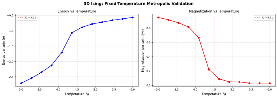
The 3D validation confirms:

Phase transition occurs near $T_c \approx 4.51$
Same qualitative behavior as 2D
Implementation is correct and ready for SA optimization

5. Simulated Annealing for 3D Ising

Now that we've validated our implementation, let's use Simulated Annealing to optimize the 3D Ising model: finding the ground state configuration.

SA Implementation

We'll use a geometric cooling schedule: $T_{k+1} = \alpha T_k$ where $\alpha = 0.98$ (slow cooling).

class GeometricSchedule:
    """Geometric cooling schedule: T_{k+1} = alpha * T_k"""
    
    def __init__(self, T0, T_min, alpha=0.95):
        self.T0 = T0
        self.T_min = T_min
        self.alpha = alpha
        self.T = T0
        self.k = 0
    
    def get_temperature(self):
        return self.T
    
    def cool(self):
        self.T = max(self.T * self.alpha, self.T_min)
        self.k += 1
    
    def is_done(self):
        return self.T <= self.T_min


def simulated_annealing_3d(ising, schedule, sweeps_per_T=10, seed=None):
    """Run Simulated Annealing on 3D Ising model.
    
    Args:
        ising: Ising3D instance
        schedule: Cooling schedule (GeometricSchedule)
        sweeps_per_T: Number of sweeps at each temperature
        seed: Random seed
    
    Returns:
        Dictionary with history (energies, temperatures, acceptance_rates)
    """
    if seed is not None:
        np.random.seed(seed)
    
    energies = []
    temperatures = []
    acceptance_rates = []
    
    while not schedule.is_done():
        T = schedule.get_temperature()
        
        # Run sweeps at this temperature
        for _ in range(sweeps_per_T):
            acc_rate = metropolis_sweep_3d(ising, T)
            energies.append(ising.get_energy_per_spin())
            temperatures.append(T)
            acceptance_rates.append(acc_rate)
        
        schedule.cool()
    
    return {
        'energies': np.array(energies),
        'temperatures': np.array(temperatures),
        'acceptance_rates': np.array(acceptance_rates)
    }

Running SA

L = 12  # System size
J = 1.0
T0 = 6.0  # High starting temperature
T_min = 0.2
alpha = 0.98  # Slow cooling
sweeps_per_T = 10

# Ground state energy per spin
E_ground = -3 * J  # All spins aligned in 3D

# Create system
ising = Ising3D(L, J=J, random=True)
E_init = ising.get_energy_per_spin()

# Run SA
schedule = GeometricSchedule(T0, T_min, alpha=alpha)
results = simulated_annealing_3d(ising, schedule, sweeps_per_T=sweeps_per_T, seed=42)

E_final = ising.get_energy_per_spin()

Output:

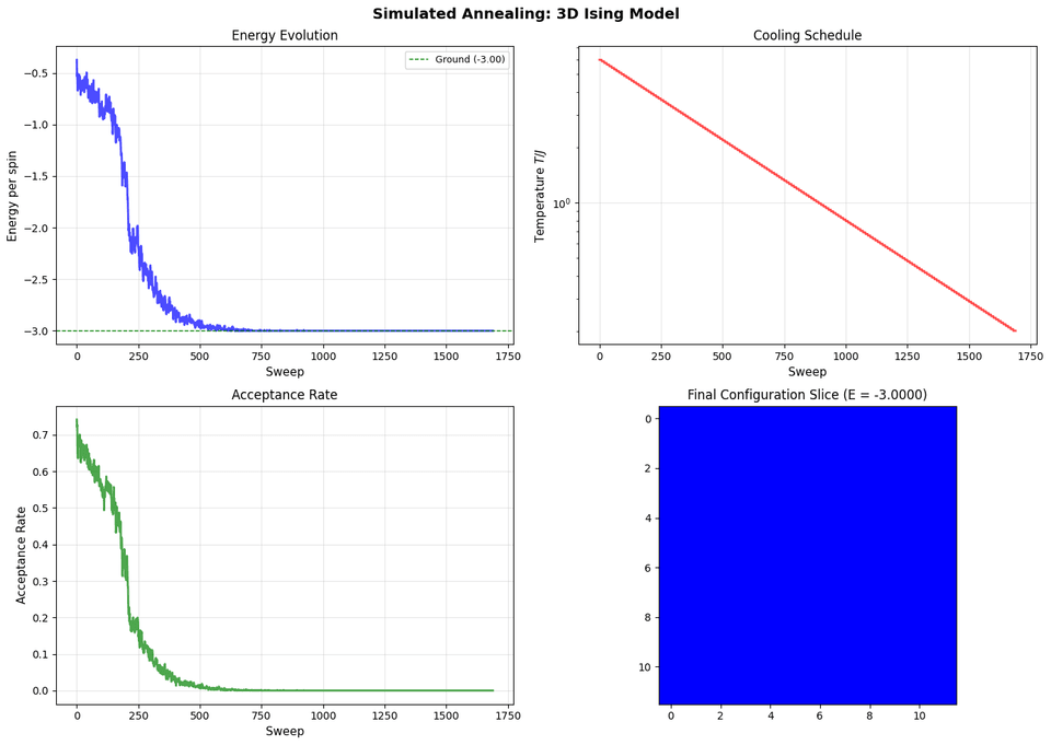
Key Characteristics of SA on Ising Model

Energy Evolution:

Starts high (random configuration)
Decreases gradually as temperature cools
Approaches ground state energy

Temperature Schedule:

Starts high: Allows exploration (accepts many uphill moves)
Decreases gradually: Transitions to exploitation
Ends low: Mostly accepts downhill moves

Acceptance Rate:

High at start: Many moves accepted (exploration)
Decreases with temperature: More selective (exploitation)
Low at end: Only good moves accepted

Configuration Evolution:

High T: Disordered, many small domains
Medium T: Larger domains form
Low T: Mostly ordered, few domain walls

Comparison with Fixed-T: SA finds lower energy than fixed-temperature Metropolis because it allows the system to explore at high temperature, then gradually settle into low-energy states.

6. Closing

I hope you enjoyed this journey through the 3D Ising model and Simulated Annealing as much as I did! This is a perfect example of how physics can be used to solve hard optimization problems.

I've been wanting to explore the Ising model for a while now, and this project was a great way to do it. I may write a follow-up post using Simulated Annealing to solve other optimization problems, but this feels like a solid foundation to build on.

References

Onsager, L. (1944). Crystal statistics. I. A two-dimensional model with an order-disorder transition. Physical Review, 65(3-4), 117-149. — Exact solution for 2D Ising model
Binder, K., & Heermann, D. W. (2010). Monte Carlo Simulation in Statistical Physics: An Introduction. Springer. — 3D Ising critical temperature $T_c / J \approx 4.51$
Kirkpatrick, S., Gelatt, C. D., & Vecchi, M. P. (1983). Optimization by simulated annealing. Science, 220(4598), 671-680. — Original Simulated Annealing paper
Metropolis, N., et al. (1953). Equation of state calculations by fast computing machines. The Journal of Chemical Physics, 21(6), 1087-1092. — Original Metropolis algorithm